22 posts tagged with "The Key of Huanche"

A Technique to Quilting Gradient Noise

目的​

我想在一個 torus 的空間中使用演算法生成地形 (Procedural generation)，因此演算法必須使地圖邊界無接縫 (Seamless)。

被排除的方案​

The image quilting​

該算法的原理是在兩張貼圖的交界處做重疊 (overlay)，並使用 error 值尋找最短路徑而達到縫合的目的。^{1 2}

但是該算法的目的是從原始貼圖中抽出拼貼塊 (patches)，並用拼貼塊重新製作圖片，並不適合用於兩個固定邊界的縫合。

當我試著用這個算法處理 noise map 的交界會變成這樣：

Periodic Perlin Noise​

Perlin Noise 的產生是透過在網格中指定隨機的向量來創造梯度，再透過內插來生成最終的 noise map。

因此只要兩個邊界使用同一組向量，就能生成無接縫的 noise map。³

不過我個人不太想重新實做 noise 生成層級的演算法；加上雖然我的目標是生成無接縫的 noise map，但是很有可能實際上會需要縫合兩張算法完全不同的 noise map，再加上交界處很有可能不具有完整的網格（貼圖的大小不是 lattice 的整數倍），所以最終不考慮這個方案。

演算法​

其實就是做線性內插：

只是線性內插本質上就是加權平均數，這會使 noise map 變得模糊，因此加上一個修飾：

smoothstep 函數能夠增加 noise 的對比來修復部份因為線性插值造成銳利度降低（模糊）的區域。

沒有 smoothstep：

加上 smoothstep：

Evaluate resources​

We can evaluate scarcity of resources intuitively; the more rare it is, the more value it is. But scarcity of economics are measured by supply and demand, it can't be a unit which had clearly definition. We can get probability of resources generated on map, but the probability wasn't enough to measured agent, it needed been processed additionally.

Shannon Entropy and Shannon Information​

The nature of Shannon entropy is mathematics quantity which well known "uncertainty of phenomenon".¹

and $I$ is Shannon Information, it be defined as:

We can noted the meaning of $-\log_2 p_i$ is "the lower the probability of an event, the greater the information carried when the event occurs", so Shannon entropy is expected value of Shannon information, can be express by:

Formula of Crafting​

To describe pattern of items changes easily, which caused by crafting or another mechanism in the game, I borrow the form of chemical equation:

$a,b,c$：amount of materials or products $X,Y$：materials, items would vanished after crafting process $Z$：products $P$：the path of crafting, item(s) won't vanished after crafting process

Information of Items​

The nature of Minecraft World are a bunch of digital data, so were reasonably considered it as a string of information, and quantify it as Shannon Entropy or Information. For a block which status was uncertain, the value is:

and $p_i$ is probability of (some type of) block generated in map, therefore we can get information of block of certain type by:

Information of Crafting​

It could calculation entropy of nature resources by probability of generated in the map, but most of items are obtained by crafting in Minecraft, when I mention "crafting" are meaning "the mechanism can be expressed by formula of crafting in the game". Need to gain entropy of non-nature items through calculation.

Let do a crafting example:

$X,Y,W$ represents three different types of blocks, can be treated as three randomly independently event, and their probability of exists in map are $p_X, p_Y, p_W$, so we can get probability of event $Z$ happened was multiplied by probabilities, also was summing by information of probabilities:

The Ratio Between Material(s) and Product(s)​

When the ratio isn't 1, total number of items would changed.

and:

Crafting Path​

The item(s) won't vanished as crafting path in the process, so:

Multiple Crafting Path​

When there are multiple path to gain item(s), it can been treats as a parallel system, therefore, the information of products can be expressed by:

The Items with Zero Entropy​

The probability of items dropped by monster, are affected by probability of monster generation, and its not related space, but time, so:

or consider it could been generated in infinity time, the probability of generation is 1, therefor:

Information of Environment​

We must define "system", when quantified information of system, so need to defined a range of space and how many blocks or items contained in the space.There are 3 kind of definition of system which common been used under below:

1. Complete System
   • Blocks, items in inventory block, item entity dropped and items in player inventory, which contained in a limited space.
2. Block System
   • Blocks and items in inventory block, which contained in a limited space.
3. Player System
   • Items in the player inventory.

We can quantify entropy of system through rules has been created, and intervening variables can been gain by making statistics on map. We can expect the entropy of environment would changed through behavior of agent, therefore those changes could be one of index of evaluated the agent.

Table of Items Information​

The following information evaluation value is for reference only, there are not included every items in the game, and process are not very rigorous. The goal is demonstrated the theory of this article, anyone are interested can finished the table by self.

Natual Resource​

Using Cuberite 1.7.X-linux64² to generate map and making statistics by plugin³. There were sampling 10 times, and remove map file to generate new seed every time. To simplify data, I merged yellow flower and red flower, removed flowing water, flowing lava, cobblestone, torch, flame, monster spawner, chest and dead bush, replace them by air.

Products​

Wood Plank​

Crafting Table​

Stick​

Wooden Pickaxe​

Cobblestone​

To simplify calculation, there's not consider crafting path with another type of pickaxe except wooden one.

Furnace​

Stone Pickaxe​

Iron Ore Item​

To simplify calculation, there's not consider crafting path with another type of pickaxe except stone one.

Coal​

To demonstrate calculation of parallel system, there's consider crafting path with wooden and stone pickaxe.

Iron Ingot​

The Table​

It is summary those value are calculated or mention in this article, and just as I said, this article didn't calculated all information of items in the game, therefore the table are unfinished:

Conclusion​

Just like James Lovelock said⁴:

I’d look for an entropy reduction, since this must be a general characteristic of life.

We can quantify extropy which agent created by reform the environment, to measue the policy:

tags: The Key Of Huanche​

評價資源​

我們能夠直觀的以資源的稀有程度去抽象的衡量資源的價值；越稀有的資源越有價值，反之亦然。但是經濟學上的價值是透過供需市場產生的，並不能作為有明確定義的綱量。我們能獲得的是資源生成在地圖上的機率，但是僅有資源機率並不能夠適當直接作為 agent 的評價手段，需要一些額外的處理。

夏農熵與夏農資訊 (Shannon Entropy and Information)​

夏農熵本質上是對我們司空見慣的「不確定現象」的數學化度量。¹

其中 $I$ 為夏農資訊，被定義為：

我們可以注意到當中的 $-\log_2 p_i$ 所描述的意義為：「事件發生的機率越低，則當該事件發生時所夾帶的資訊越大」，因此夏農熵也是對不確定的夏農資訊的期望值，亦可寫作：

合成式 (Formular of Crafting)​

為了方便描述合成或其他遊戲機制使資源 (items) 發生變化的過程，我借用了化學反應式的形式來表達：

$a,b,c$：原料或產物的數量 $X,Y$：原料，合成過程會被消耗的物品 $Z$：產物 $P$：合成途徑，參與合成但是不會被消耗的物品。

資源的資訊量 (Information of Items)​

Minecraft 世界在本質上就是一團數位資料，因此將其視作一串由方塊構成的資訊，並用夏農熵或夏農資訊去衡量其資訊量是十分合理的作法。對於一個不確定狀態的方塊來說，其值為：

其 中$p_i$ 為某種類型的方塊出現在地圖中的機率，換句話說我們可以得知特定種類方塊其資訊量為：

合成的資訊量 (Information of Crafting)​

天然資源能夠以其在地圖生成的機率來計算熵，但是 Minecraft 中的大部分物品需透過合成途徑獲得，當我提到合成是指：「能夠被合成式所表示的所有遊戲機制」，這些非天然物品的熵需透過計算取得。

以一個合成為例：

$X,Y,W$ 分別代表三種不同類型的方塊，我們可以視作三個隨機事件，而這三者出現在地圖的機率分別為 $p_X, p_Y, p_W$ 並且互為獨立事件，因此我們可以得知事件 $Z$ 發生的機率為三者的機率相乘，也就是三者資訊量的加總：

數量的變化 (The ratio between resource and product)​

當原料與產物的比值不為 1 時，物品的總數量發生了變化。

則：

合成途徑 (Crafting Path)​

作為合成途徑的物品不會被消耗，因此：

多重途徑 (Multiple Crafting Path)​

當一個物品有多種取得途徑時可以視作一個並聯系統 (parallel systems)，因此該物品的資訊量可以寫作：

零資訊的資源 (The Items with Zero Entropy)​

怪物掉落物仰賴怪物的生成，但是怪物生成的機率並不是與空間關聯，而是與時間關聯的，以空間機率考慮：

若或是考慮其在無窮的時間中能夠被無限生成，事件發生的機率為 1，因此：

環境的資訊量 (Information of Environment)​

當我們要量化系統的資訊量時，必須先界定所謂的「系統」。要定義一個系統，我們要給定一個範圍（空間大小）以及具體包含了多少方塊或物品。以下有三種定義應該是我們比較常用的系統類型：

1. 完整系統
   • 在一劃定的範圍內，所包含的方塊、收納方塊內容物、掉落物與玩家物品欄（裝備欄）內容物。
2. 方塊系統
   • 在一劃定的範圍內，所包含的方塊與收納方塊內容物。
3. 玩家系統
   • 玩家物品欄（裝備欄）內容物。

透過到目前為止建立的規則，我們可以量化一個系統的熵，而該值能透過統計地圖中的方塊與實體取得。隨著 agent 在環境中活動，我們可以預期環境的熵會因此發生改變，這個變化量便可做為評量 agent 的指標之一。

資訊量表 (Table of Items Information)​

以下的資訊量評估值僅供參考，過程並不嚴謹並且沒有對所有的物品進行計算。目的只是透過實做示範如何實踐本文建構的理論，有興趣的人可以自行用更嚴謹的方式建構完整的遊戲物件資訊量表。

天然資源 (Natual Resource)​

使用 Cuberite 1.7.X-linux64² 生成地圖並搭配插件³統計方塊數量。總共抽樣 10 次，每次都會將地圖檔案刪除以生成新的種子。為了簡化數據，將紅花與黃花視為同樣的東西，並將流動水、流動岩漿、鵝卵石、火把、火焰、生怪磚、箱子與枯萎灌木移除並用空氣取代。統計資料如下表：

加工品 (Products)​

木板​

工作台​

木棒​

木鎬​

鵝卵石​

為了簡化計算，下列過程不考慮其他材質的鎬挖掘的情況。

熔爐​

石鎬​

鐵礦​

為了簡化計算，下列過程不考慮其他材質的鎬挖掘的情況。

煤​

為了示範並聯系統的計算，以下僅考慮木鎬與石鎬的挖掘途徑。

鐵錠​

資訊量總表 (The Table)​

正如我提過得，本文並沒有計算所有物品的資訊量，僅是將先前統計或計算得到的數值做個整理，因此這個表並不完整。

結語​

就如像詹姆斯·拉夫洛克(James Lovelock)所說的⁴：

I’d look for an entropy reduction, since this must be a general characteristic of life.

我們可以透過 agent 對環境進行改造從而造成的熵減量，作為衡量策略的方法：

實驗紀錄​

實驗摘要​

• 實驗日期
  • 2020-03-22
• 實驗內容
  • 同樣使用 opencv 的函式庫，但是控制變因如下：
    1. 直接傳輸 bitmap，並建立 cv::Mat
    2. 傳輸 png 再解碼建立 cv::Mat

實驗結果​

Connecting to opencv server with bitmap…
average time during:  0.0010088205337524414
Connecting to opencv server with png…
average time during:  0.008921647071838379

實驗結論​

推測：

• 資料轉換成 std::vector<char> 與解碼的過程花費多餘的時間
• 測試發生在本地，網路傳輸的成本本來就比較低，在網路瓶頸的環境表現出的優劣可能會不太一樣

有一個討論串跟我的問題相同，並且在當中提到，png 編碼與解碼本身就會花費不少時間，資料傳輸方式的選擇還是要根據環境的硬體設備情況去做調整¹。

The Nature Of Intelligence​

What is intelligence?

That's the question which many people working on artificial intelligence would asked. Let standing at the basic of natural science to look this question.

Thermodynamic arrow of time​

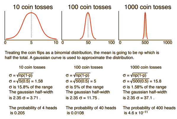
The arrow of time is the "one-way direction" or "asymmetry" of time. The thermodynamic arrow of time is provided by the second law of thermodynamics, which says that in an isolated system, entropy tends to increase with time. Entropy can be thought of as a measure of microscopic disorder; thus the second law implies that time is asymmetrical with respect to the amount of order in an isolated system: as a system advances through time, it becomes more statistically disordered. This asymmetry can be used empirically to distinguish between future and past, though measuring entropy does not accurately measure time. ¹ So there for would be consequent between past and future, "cause" and "effect" .

Mapping Relationship Between Cause And Effect​

The relationship between cause and effect can be written by boolean function as below:

Intelligence of creatures​

The intelligent creatures just a logical system to make reaction with environment information, which the nature of intelligent is a mapping relationship, the informations from environment are cause and the reactions of creature made are effect. So we can express intelligence of creatures by boolean function but huge and complicate.

Neural Network​

It's undeniable that artificial neural network had flexibility which creating many kind of logical mapping relationship, but the artificial neural network that based floating point arithmetic cause many information losing, computer cost too many time and energy to calculating the information that we don't needed.

Of course there are information also loses in boolean calculation, but it necessary process which extracting value information for agents, and unliked artificial neural network, boolean algebra had more interpretability, we can translate relation between input and output.

There for, why not to use both of artificial neural network and boolean algebra? This is a formula of neuron of artificial neural network:

and its formula of neuron of BNN (boolean neural network):

Why Don't Just Using Logic Array?​

Because BNN have some properties which logic array don't had: Logic array cannot contain recurrent structure (memory unit). But major problem is interpretability, as know as the hidden layers in the artificial neural network can be explained as extracting features and provided more specific concepts, there for logic array cannot provided tree structure to do that.

General Logic Unit​

Just like biology, we observe subjects and make inductive science system to study them. There might reasonably be expected from some patterns of BNN occurred repeatedly and been observed, that means those patterns are GLU (generic logic unit). When we had created knowledge base of GLU, would allow us to explanation how BNN "thinking".

tags: The Key Of Huanche​

智能體的本質​

What is intelligence?

這是許多從事人工智慧研究的人會問的問題。 讓我們站在一些基本的自然科學前提上看待這個問題。

熱力學時間箭頭​

熱力學時間箭頭來自熱力學第二定律，這一定律認為一個孤立系統的熵只能隨著時間流易不斷增加，而不會減少。熵被認為是無序的量度，因此第二定律隱含著一種由孤立系統的有序度變化所指定的時間方向（也就是說，隨著時間流易，系統總是越來越無序）。這種不對稱性可用於區分過去和未來¹，因此產生了因果關係。

「因」與「果」的映射關係​

因果之間的映射關係可以用布林函數表示，如下：

or

其中：

• C: 因
• E: 果

生物的智能​

生物的智能只是一個與環境信息發生反應的邏輯系統，智能的本質是一種映射關係；來自環境的信息是因，而生物的反應則是果。 因此，我們可以通過大型且複雜的布爾函數來表達生物的智能。

神經網路​

不可否認，人工神經網絡具有創建多種邏輯映射關係的靈活性，但是其基於浮點數定義的算法導致許多資訊丟失，計算機花費大量的時間和算力在在計算我們最後沒用到的資訊。

當然在運算布林代數時也有資訊會丟失，但是這是萃取有價值的訊息的必要過程，與人工神經網絡不同，布林代數具有更多的可解釋性，我們可以翻譯輸入和輸出之間的關係。

為什麼不同時使用人工神經網絡和布爾代數呢？ 這是人工神經網絡的神經元公式：

然後這是 BNN（boolean neural network）神經元的公式：

何不使用邏輯陣列？​

因 BNN 具有邏輯陣列所沒有的一些特性：邏輯陣列結構上沒有遞歸 (recurrent) 的功能。 但是主要的問題是可解釋性，眾所周知人工神經網絡中的隱藏層可以視作抽取特徵的過程，並透過組合低級特徵成為更高級的特徵或是從抽象概念組合成更具體的概念，然而邏輯陣列並沒有樹狀結構來實現這一點。

通用邏輯單元​

就像生物學一樣，我們觀察對象並建立歸納科學系統來研究它們。可以合理地預期會觀察到某些模式會重複出現在 BNN 之中，這意味著這些模式是 GLU （通用邏輯單元）。 當我們創建了 GLU 的知識庫時，使得我們能夠透過這些邏輯單元去解釋 BNN 是如何進行思考的。

拓撲進化類神經網路 (NEAT) ，必定有會自然演化出遞歸 (recurrent) 結構，若不能妥善處理遞歸衍生的問題，演算法就不能完備。下圖是一個遞歸結構的範例：

不難看出它是一個遞迴構造，最大的問題就是如何處理遞歸連結造成的遞迴？有一種方式是規定遞迴深度（次數）¹，或是將整個網路的連接都定義為遞歸連結²。

類神經網路拓撲結構的數學定義​

類神經網路是以抽象連結的方式存在，即使為了視覺化而把網路成現在平面或立體中， 這些連結的長度與神經元之間的距離並不影響神經網路的性質， 因此類神經網路存在於拓撲空間而不存在於度量空間，又或是說類神經網路具有拓撲性質。

首先我們定義有序對（Ordered pair）³，之後要用來處理有向圖（directed graph）的連結：

定義這個的作用是什麼？拓撲學會大量使用集合論，但是如果我們把連結的頭尾單純丟到一個集合中，如： $a = {x_1,x_2}$ ，並不能描述誰是頭誰是尾，而只能描述條連結線而已，所以定義一個能夠對兩個元素產生後差異的數組十分重要。

定義一張有向圖 (Directed Graph)⁴：

V：頂點集（vertices set），紀錄了所有點

A：連結集，紀錄了點與點的有向連接（箭頭,arrow）

W：權重集，紀錄了連結的權值

拓撲排序​

對一個有向無環圖 (Directed Acyclic Graph) 而言，它是可以被排序的：

當拓撲結構被排序後，就有了前後的相對關係，如此一來我們就能判斷連結究竟屬於前饋的還是遞歸連結。呼叫遞迴時，連結由前往後傳遞時呼叫遞迴產生新值；由後往前傳遞時則回傳舊值，。

但是拓撲排序只適用於無環的結構，當圖上有環，拓樸順序就不存在。因為環上每一個點都會有連向自己的邊，意味著環上每一個點必須排在其他點的後方，環上每一個點都不能在排列順序中拔得頭籌，所以合理的排列順序不存在。⁵

那麼假若拓撲結構一開始就定義了順序呢？

如此一來在任一節點呼叫遞迴，必然存在中止條件。實做的時候也很方便，可以直接沿用節點的編號作為拓撲排序的依據，而不需要額外的變數來處理遞迴中止條件。

Wei Ji以創用CC 姓名標示-相同方式分享 4.0 國際 授權條款釋出。

給定類神經網路輸入與輸出節點的數量，並給定資料集的前提下，究竟要設定多少隱藏神經元才能完成任務？這個問題可以理解成：

在已知環境；且任務明確的前提下，智能體要具有多少資訊才能完成任務？

當環境本身的資訊量非常龐大時，我們無法量化環境究竟具有多少資訊的情況，似乎也無法計算出智能體究竟需要多少資訊才能完成任務。綜觀生物演化，想必不是「先設想需要多少基因」再演化出能夠活下來的生物，而是「能夠活下來的生物自然擁有這麼多的基因」，因此隨著訓練過程同時嘗試較多神經的網路與較少神經的網路，最後能達成任務的網路大小就是好的網路大小。

基因編碼​

一個布林類神經網路可以用一段染色體描述，染色體區分成兩個部份：

• 定址基因
• 連結基因

定址基因決定這個網路擁有多少節點，換言之，決定網路的大小。連結基因則是描述兩個節點之間的連結。

定址基因​

決定熵庫大小的基因。若定址基因儲存的變數為 $n$，則網路具有 $2^n$ 個節點，因此在定址基因為 1 byte 的前提下，本基因算法的定義最多可以描述有 $2^{256}$ 個節點的布林類神經網路。

連結基因​

一段連結兩個類神經元節點的資訊可以被描述為：

• $a$ : address， 連結的定址， 訊號將會從 $a_1$ 送往 $a_2$
• $w$ : weight，權值，決定訊號邏輯是否會被反轉

因此一段用來描述連結的基因有三個部份：

• 來源節點
• 目標節點
• 權值

基因資料空間用量​

資料應該儲存為文字檔案 -- The UNIX Philosophy¹

使用二進制編碼的染色體檔案會無法直接被人類閱讀，這其實是有違 Unix 哲學的，若沒有良好的理由應該避免這麼做。因此接下來試著計算這麼做在資料壓縮上的利益。

若一網路以 100 萬畫素相機作為輸入：

• RGB -> 3 個 100 萬矩陣
• 一個色彩值 0~255 -> 每一個單色像素花費 8 bit 的資料

總計 24,000,000 個布林輸入：

布林類神經網路理論要求至少要4層網路

• 1層輸入層
• 2層隱藏層
• 1層輸出層

假設輸出值只有一個位元，因此先不考慮輸出層，總計需要 72M 個節點：

即定址空間至少為 27 位元：

則一個連結至少需要多少資料表達：

若使用字串描述十進制，則連結資訊至多會消耗 9 位數，平均消耗 8 位數：

若使用字串儲存（十進制）， [定址1][定址2][權值][分割字符]

不過目前多使用 UTF-8 編碼，因此儲存空間會變成兩倍: 288 bit， 結論：使用二進制定義的資料壓縮率為 0.19

突變機制​

任一染色體經過突變之後會得到新的染色體：

$G'$: 後代染色體，為隨機變數 $G$: 染色體 $m$: 突變率，或為複製失敗的機率

定址基因​

對染色體而言，定址基因有 $m$ 的機率會複製失敗， 而失敗時又有 0.5 的機率會增加； 0.5 的機率會減少， 因此當定址基因突變時，有一半一半的機率會加一或是減一， 從而觸發「定址擴張」或「定址萎縮」的事件。

連結基因​

參考染色體的異常模式²：

• deletion
• duplication
• inversion

考量 inversion 的破壞性，只保留前面兩者突變機制，因此對一段基因而言，突變的機制有兩種：

• 刪除
• 複製

複製可以用來探勘解；刪除則可以用來收斂解。 對基因而言，有 $m$ 的機率會複製失敗，當複製失敗時有 0.5 的機率發生刪除；0.5 的機率發生複製。

位元突變​

位元突變是每一個位元的基因在複製給下一代時， 皆有一定機率 $m$ 會發生複製錯誤，即邏輯反轉。

透過基因複製與位元突變，便可產生不同的連結基因並增加網路的連結進而曠大網路的大小。

定址擴張與萎縮​

當定址基因發生突變時，整個網路的熵庫就會發生擴張或是萎縮。我們通常將輸入放置在拓撲排序的前方而輸入放在後方，因此當網路方生擴張時，會將原生的網路資訊一分為二，將後段部神經元的編號映射到新的熵庫後方。萎縮時則反向操作，與中間節點有關的所有連結資訊都會被刪除。

Wei Ji以創用CC 姓名標示-相同方式分享 4.0 國際 授權條款釋出。

熵—衡量萬物混亂程度的物理量...嗎？​

熵 (Entropy) 具有很多種表述方式，比如：

• 克勞修斯熵 $d S = \frac{\delta q}{T}$
• 波滋曼熵 $S = k \ln W$
• 資訊熵（夏農熵） $S = \log_2 2^N = N$

有一種熵的詮釋與「狀態所包含的排列數」相關，波滋曼熵與夏農熵便是如此。以波滋曼熵為例，當中的 W 所代表的意義是微觀物理的狀態數¹：

夏農熵中 $2^N$ 則是在 N bit 的空間中；資訊有幾種排列方式。夏農熵有另外一種表述方式²，在此就先不贅述。

總之先擲點硬幣吧！​

現在想像一個盒子內裝有 n 枚硬幣，當我隨意上下搖晃盒子，內部的硬幣就會以一半反面一半正面的機率翻面。

我們可以發現 k 枚硬幣正面朝上的排列數可以寫作：

以 n=10 為例，我們對 W(k) 作圖：

我們可以發現當 $k=\frac{n}{2}$ 的時候排列數最多，若依照熵的定義；此時的熵應該也是最大的。

熵的相對性​

雖然特定狀態的排列數可以定義出該狀態的熵值，但是實務上我們考慮的是「熵的變化」：

畢竟當系統十分龐大時，你很難計算或窮舉出它的所有可能的排列（數）。

機率使其往高熵發展​

根據經驗，我們知道隨著搖晃盒子，硬幣正面、反面朝上的分佈應該會是一半一半。但是我們如何用數學解釋這個現象呢？

這個將硬幣放在盒子內的實驗，可以視作伯努力試驗，而伯努力試驗又可以用二項式分佈來描述：

$k$：成功的次數，在本例的情況是指正面朝上的硬幣數目 $n$：進行試驗的次數，在本例的情況是指總共有多少枚硬幣 $p$：成功的機率，在本例就是正面朝上的機率，也就是 0.5 $\Pr$：機率密度

³

二項式分佈若繪圖會得到上述圖形，y 軸是機率密度，x 軸則是 k 值。可以看到它的分佈趨近常態分佈。根據二項式分佈的特性我們可以得到其標準差為：

隨著 n 增大，其標準差佔整體的比例會越來越窄⁴：

若考慮 1,000 枚硬幣，標準差為 15.8 ，跨越 3 個標準差的距離為 453 ~ 547，這代表有 99.7% 的機率，正面朝上的硬幣數量會在 453 ~ 547 這個區間內。

若考慮 1,000,000 枚硬幣，標準差為 500 ，跨越 3 個標準差的距離為 498,500 ~ 501,500，這代表有 99.7% 的機率，正面朝上的硬幣數量會在 498,500 ~ 501,500 這個區間內。

我們可以發現當 n 增大，機率分佈會聚集在少數的某些狀態，而其他狀態發生的機率便顯得微乎其微。

有人說熵就是亂度？​

我們可以注意到機率分佈會集中在 $k=\frac{n}{2}$ 附近，而 $k=\frac{n}{2}$ 時又是熵最大的狀態，因此我們可以注意到熵越大的狀態越容易自然發生。

不管我怎麼排列這些硬幣，只要隨著搖晃盒子，硬幣的分佈都會往熵最大的狀態發展。令我排列的狀態熵為 $S_0$ ，而最終狀態的熵為 $S_1$ 則：

不論你從何種狀態往最終狀態變化，其 $\Delta\,S$ 必定大於 0。這就是熱力學第二定律。

當我們排列硬幣時，會下意識的將該狀態視為「有序」，而經過搖晃盒子後，硬幣的分佈狀態則下意識地視作「混亂」，因此看似萬物都會自然往混亂發展，如此以來熵似乎就和混亂掛勾了，似乎熵能夠描述事物的「混亂程度」。「秩序」與「混亂」的狀態其實是相當抽象且無法被明確定義的，「熵代表著混亂的程度」是一種通俗的理解方式，但是也是相對不嚴謹的理解方式。

資訊的不確定性與熵的關係​

我們來看看兩組資料，其中 x 代表可以為 1 也可以為 0 ，是一個不確定的資料：

1. 10101010
2. 10x01x10

根據熵與排列數之間的關係，我們可以發現第一組資料的排列數只有 1 種，後者的排列數則有 4 種，也就是後者的熵較高。

資訊體生物的空想實驗​

首先想像一個資訊生物，其所承載的資訊會影響這個生物的各種性狀 (Phenotypic trait)，它的資訊是完全明確的，並且任一位元的資訊發生變化就會造成系統異常（遺傳疾病）從而造成生物整體的崩潰：死亡。

接著想像另外一個資訊生物，他有部份的資訊是不確定的，也就是資訊為 1 還是 0 所表現出的性狀皆不會對本體造成關鍵的危害。

想像這兩隻資訊生物被放置於同一個環境之中，前者因為不容許任何錯誤，其後代資訊一定是完全複製的，因為複製錯誤的都會死亡；另外一隻的後代則容許一定程度的變化，這個變化也包含資訊數變多。

不難想像在長時間的迭代中，後者遲早會發展出更多的競爭競爭優勢。如果兩種生物處於相同的環境之中，不會（無法）發生變化的資訊生物會漸漸的在競爭中消失。

熵庫 (Entropy Reservoir) 與熵池 (Entropy pool)​

資訊生物的資訊都能夠被描述成不確定的部份以及確定的部份，如：

並且任意資訊都能被母體集合 $P$ 包含：

這個 $P$ 就是熵庫 (Entropy Reservoir)，理想熵庫是一個無限大的集合，而且充滿了不確定的資訊。被資訊生物收錄的不確定資訊則稱為熵池 (Entory Pool)，任何能夠描述具有競爭優勢的性狀的資訊皆來自不確定資訊的收斂。

描述競爭優勢的確定資訊必須由熵池中的不確定資訊收斂而來；不確定資訊則必須從熵庫獲得。 我們可以將獲得資訊的過程想像成一種開採資源的過程，這種資源必須從不確定資訊收斂而來，而不確定資訊又必須從熵庫中開採，並且整個過程消耗著時間與能源。

Wei Ji以創用CC 姓名標示-相同方式分享 4.0 國際 授權條款釋出。

首先考慮一個具有記憶能力的邏輯單元（也許是RNN）， 它的輸出 $g(t)$ 受到當前輸入 $f(t)$ 與先前部份輸出 $g_B(t-1)$ 的影響。

我們可以透過一個空想實驗來理解這個過程：

1. 今天我看到小明吃蘋果

"小明吃蘋果"這段資訊就是 $f(0)$ ，但是我並不會因為這個資訊而特別做出什麼行為，僅僅只是記著。

2. 隔天我又看到小明吃蘋果。

隔天看到"小明吃蘋果"這段資訊就是 $f(1)$，而"小明昨天也吃蘋果"就是 $g_B(0)$，把這兩個資訊揉合在一起，我產生了新的概念"小明連續吃了兩天的蘋果"；這就是$g_B(1)$

3. 如此一般持續過了一個月，小明幾乎天天吃蘋果。（爾偶不吃）

究竟哪一天小明有沒有吃蘋果，我並不會清楚的記得，而是變成"小明過去一個月經常吃蘋果"這樣一個概念記在腦海中，而這個概念就是 $g_B(30)$。

4. 小明今天心情似乎很糟，而且還沒見他今天吃蘋果。

"小明心情很糟，沒吃蘋果"這個資訊就是 $f(31)$。

5. 於是我買了蘋果送給他

"買蘋果送他"這個觸發行為的指令就是 $g_A(31)$。

當然，這是一個簡化的空想實驗，以天為最小時序單位、一些邏輯映射關係也直接省略（如："買蘋果送他"這個輸出似乎還應該夾帶"別人不開心我也不開心"或"小明對我而言是個特別的人"...之類的其他輸入資訊才能發生的邏輯映射。

只是為了方便讀者釐清幾個簡單的概念：

1. 智能體的當前決策，來自當前認知以及先前記憶造成的邏輯映射。
2. 資訊會被壓縮並丟失。
3. 資訊的壓縮與丟失不只發生在認知，也發生在記憶。
4. 因此智能體不會 100% 的記憶所有細節。

輸入資訊量、記憶資訊量與資訊損失之間的關係​

接著我進行了幾個假設：

1. 所有輸入與輸出的資訊都是二進制的數組
2. 只在乎資訊的量，而不在乎內容，也就是數組的位元數
3. 輸入的資訊量不隨時間改變( $\forall t:F=F(t)$ )

於是我列出了下式：

$G$：輸出的資訊量，也就是位元數 $F$：輸入的資訊量 $\eta_1,\eta_2$：資訊殘留率，其值小於等於1

對任意時間而言的輸出資訊量，來自於當前輸入資訊量流失；以及先前輸出的資訊流失後的加總。

於是我們可以列出：

可以歸納出：

若考慮在無窮的時間後，智能體被資訊塞滿的情況：

資訊殘留率的測定​

對任意輸出位元 $g_i(t)$，其值決定於 $f(t)$ 與 $g(t-1)$ 的布林函式。

固定 $g(t-1)$ 後窮舉 $f(t)$ ，輸出可能的排列組合數比上輸入的排列數，即為$\eta_1$：

固定 $f(t)$ 後窮舉 $g(t-1)$ ，輸出可能的排列組合數比上輸入的排列數，即為$\eta_2$：

※ "$\#$" 是集合元素數量的意思。

如果資訊位元數過高，窮舉成本過大，或許可以用抽樣的方式處理。

關於資訊殘留率​

理工的朋友看到 $\eta$ 這個記號應該會很容易連想到功率， 但是最初在設計變數的時候我是想使用 $\lambda$ 作為記號的， 畢竟它經常被使用在「衰減」的場合，而這是一個資訊衰減的場合， 不過半衰期的方程式是指數型態的，而我想描述的是一組線性方程式。

另外一個候選方案是沿用電腦科學領域已經有的資訊壓率，但是很遺憾的， 資訊壓縮率的定義與我期望使用的殘留率剛好是倒數關係； 資訊壓縮率是一個大於 1 的數值。

值得一提，還有另外一個與資訊殘留率接近但是本文並沒有使用到的概念， 生存函數（Survival function），它是一個隨著時間衰減， 並且介於 0 到 1 之間的函數，不過它的衰減模式是一個變化的過程， 而且考慮的是連續的時間。（本文的模型是離散的，而且衰減模式固定）

衡量智能體的智能程度​

我的目的是為了分析布林類神經網路才建立這個模型的， 不過仔細想想，這個模型好像能描述各種「具有記憶能力的智能體」。

智能體基本上是一個映射函數，反應輸入到輸出之間的映射關係， 而在此模型中，為了簡化問題，所有映射關係都由布林運算完成。

$F$：輸入智能體的資訊量，單位為 bit $G_A$：輸出智能體的資訊量，單位為 bit $G_B$：記憶於智能體的資訊量，單位為 bit $\eta$：資訊殘留率

注意，資訊量描述的並不是有幾條線。舉例來說 3bit 的解碼器，其輸出有 8 條線，但是資訊量仍為 3 bit，資訊量的定義如下：

智能體極限記憶能力評估​

透過實驗（解析布林函數）的方式可以獲得 $\eta_1$、$\eta_2$ ， 再透過公式便可計算出該智能體最多能儲存多少資訊：

理想的行為複雜度​

行為複雜度 $G_A$ 可以很直觀的列出：

接著我們把極限記憶能力 $G_B$ 代入可得：

然後我們假設：

• $f(t+1)$ 的資訊會被完全映射到 $g_B(t+1)$ ，$\eta_1=1$
• $f(t+1)$ 和 $g_B(t)$ 的資訊會完全映射到 $g_B(t+1)$ ， $\eta_3=\eta_4=1$

便會得到下式，某種程度上理想條件的行為複雜度：

這是決定智能體輸入資訊複雜度 $F$ 與記憶率 $\eta_2$ 之後，所能預期智能體的理想狀態的行為複雜度，此時的 $g_A$ 是一個對射函數。

唯獨 $\eta_2$ 不能假設為 1 的原因是，該公式的先決條件是在無窮的時間後，智能體的記憶單元塞滿了資訊，如果智能體無法忘記資訊，則 $G_B$ 會發散（智能體可以儲存無限的資訊），如此假設並沒有實際的意義。

行為複雜度​

根據公式：

我們可以透過實驗獲得資訊殘留率，而輸入資訊量 $F$ 是網路結構給定的，這樣便可測定智能體的行為複雜度。

如此一來便可將智能體在不需要仰賴模擬環境的情況下進行分析，而這個分析結果代表著「終端狀態」，比如：

• 無限的時間之後的記憶能力
• 記憶體充滿資訊的完全狀態的智能體的反應
• 終端穩定狀態智能體丟失資訊的數量
• etc.

但是我們也可以將智能體丟在環境中，取樣一段時間來評估資訊殘留率， 從而統計智能體在不同環境中，隨時間變化而產生的行為複雜度差異。

成熟假說​

在一開始的 $\eta_3$ 應該會偏大， $\eta_4$ 偏小， 智能體在記憶（學習）環境之前的反應仰賴當前接收的資訊， $G_B$ 偏小，因為沒有多少資訊被記憶。

當智能體漸漸成熟後，反應仰賴於過去經驗， $\eta_3$ 應該會慢慢變小，而 $\eta_4$ 漸漸增加。

直到 $G_B$ 到達極限，此時智能體無法再學習更多資訊了，即便有 $F$ bit 的資訊進入，但是同時也會有 $F$ bit 的資訊遺失，推導如下：

可以非常容易的理解 $G_B$ 就是網路結構賦予智能體的學習空間。

tags: The Key Of Huanche​